-----------------------------------
-----------------------------------
-----------------------------------
-----------------------------------
-----------------------------------
-----------------------------------
-----------------------------------
-----------------------------------
-----------------------------------
-----------------------------------
-----------------------------------
-----------------------------------
-----------------------------------
-----------------------------------
-----------------------------------
-----------------------------------
-----------------------------------
-----------------------------------
-----------------------------------
-----------------------------------
-----------------------------------
-----------------------------------
-----------------------------------
-----------------------------------
-----------------------------------
-----------------------------------
-----------------------------------
-----------------------------------
-----------------------------------
-----------------------------------
-----------------------------------
-----------------------------------
-----------------------------------
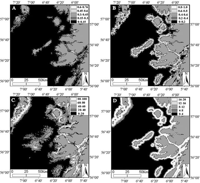
Fig. 4. Maps of predicted occurrence of harbour porpoises within the study area from each of the four modelling techniques. A. GLM – Predicted probability of occurrence for individual cells ranging from 0 to a highest probability of 0.755; B. PCA – Predicted likelihood of occurrence ranges from 0 for cells with habitat furthest from the centre of the calculated niche to 1.0 for cells with habitat closest to the centre; C. ENFA – Habitat suitability index ranges from 0 for least suitable habitat to 100 for most suitable habitat based on niche preferences calculated during analysis; D. GARP – Values range from 0-20 with 20 indicating that occurrence was predicted in all 20 runs and 0 that it was not predicted on any runs.
Source: MacLeod et al. A comparison of approaches to modelling the occurrence of marine animals.
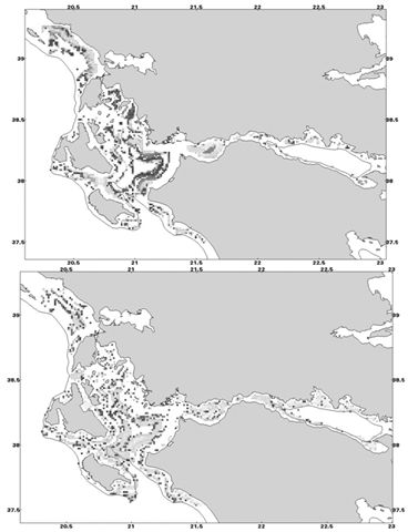
Fig. 10. General MAXENT (top) and GAM (bottom) probability map estimates for immature Illex coindetii using summer surveyed MEDITS data 1998-2006.
Source: Lefkaditou et al. Eastern Ionian Sea: Influences of environmental variability on the population structure and distribution patterns of the short-fin squid Illex coindetii (Cephalopoda: Ommastrephidae).
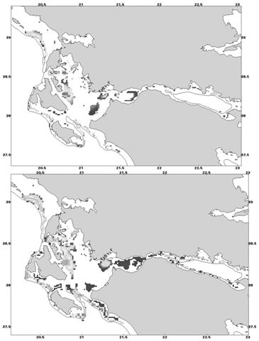
Fig. 11 General MAXENT (top) and GAM (bottom) probability map estimates for mature Illex coindetii using summer surveyed MEDITS data 1998-2006.
Source: Lefkaditou et al. Eastern Ionian Sea: Influences of environmental variability on the population structure and distribution patterns of the short-fin squid Illex coindetii (Cephalopoda: Ommastrephidae).
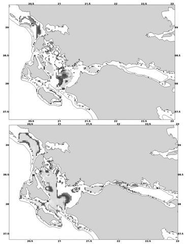
Fig. 12. General MAXENT (top) and GAM (bottom) probability map estimates for both mature and juvenile Illex coindetii using summer surveyed MEDITS data 1998-2006.
Source: Lefkaditou et al. Eastern Ionian Sea: Influences of environmental variability on the population structure and distribution patterns of the short-fin squid Illex coindetii (Cephalopoda: Ommastrephidae).
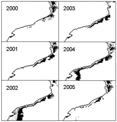
Fig. 3. GIS-based EFH maps of paralarvae Loligo vulgaris in Catalan coast (NW Mediterranean) in May 2000-2005.
Source: Sanchez et al. Combining GIS and GAMs to identify potential habitats of squid Loligo vulgaris in the Northwestern Mediterranean.
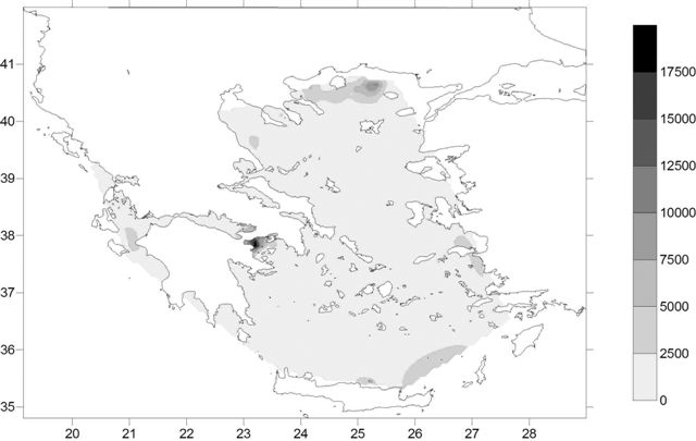
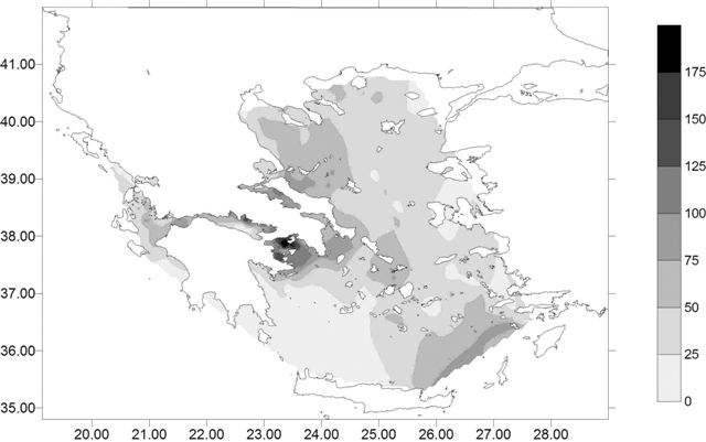
Fig. 5. Map of the total pink shrimp distribution. DI is expressed in terms of n/km2.Interpolation was made by means of the “natural neighbour” gridding method.
Source: Politou et al. Identification of deep-water pink shrimp abundance distribution patterns and nursery grounds in the eastern Mediterranean by means of generalized additive modeling.
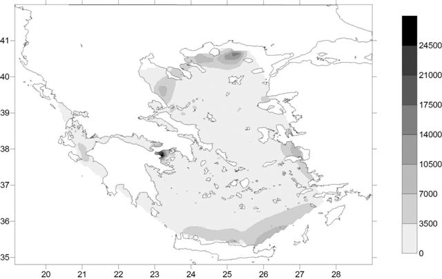
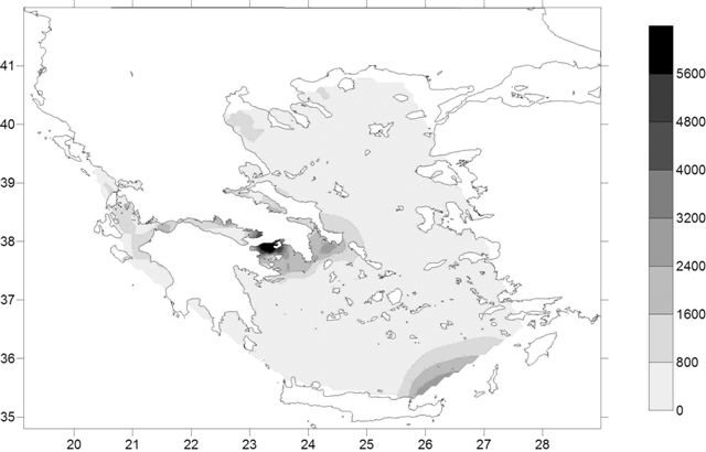
Fig. 6. Map of the adult pink shrimp distribution. DI is expressed in terms of n/km2. Interpolation was made by means of the “natural neighbour” gridding method.
Source: Politou et al. Identification of deep-water pink shrimp abundance distribution patterns and nursery grounds in the eastern Mediterranean by means of generalized additive modeling.
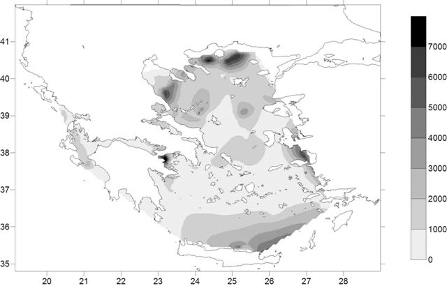
Fig. 7. Map of the juvenile pink shrimp distribution. DI is expressed in terms of n/km2. Interpolation was made by means of the “natural neighbour” gridding method.
Source: Politou et al. Identification of deep-water pink shrimp abundance distribution patterns and nursery grounds in the eastern Mediterranean by means of generalized additive modeling.
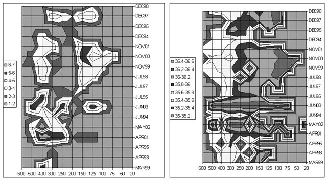
Fig. 5. Spatial distribution of spawning Parapenaeus longirostris (left) and associated salinity (right) during all surveys.
Source: Benchoucha et al. Salinity and temperature as factors controlling the spawning and catch of Parapenaeus longirostris along the Moroccan Atlantic Ocean.
efhimg/figure 5. Map of the total hake distribution. Abundance is expressed in terms of kg/km2.
Source: Tserpes et al. Identification of hake distribution pattern and nursery grounds in the eastern Mediterranean by means of generalized additive models.
efhimg/figure 6. Map of the juvenile hake distribution. Abundance is expressed in terms of n/km2.
Source: Tserpes et al. Identification of hake distribution pattern and nursery grounds in the eastern Mediterranean by means of generalized additive models.
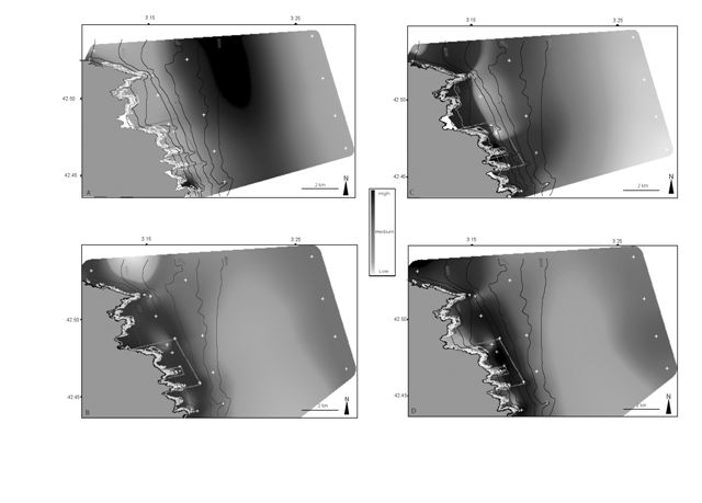
Fig. 8: Suitable Habitats in Marine Reserve of Cerbčre-Banyuls for Sparid larvae (A & B) and Scorpaenids larvae (C & D), in spring (A & C) and in summer (B & D). White dotted line area between coast and sea delimited hard (Rock and Posidonia meadow) from soft bottom (Sand).
Source: Crec’hriou et al. Spatial patterns and GIS habitat modelling of fish in two French Mediterranean coastal areas.
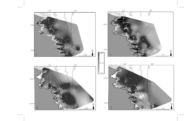
Fig. 4: Suitable Habitats in Marine Reserve of Cerbčre-Banyuls for adult Sparids (A & B) and for adult Scorpaenids (C & D), in spring (A & C) and in summer (B & D). White dotted line area between coast and sea delimited hard (Rock and Posidonia meadow) from soft bottom (Sand).
Source: Crec’hriou et al. Spatial patterns and GIS habitat modelling of fish in two French Mediterranean coastal areas.
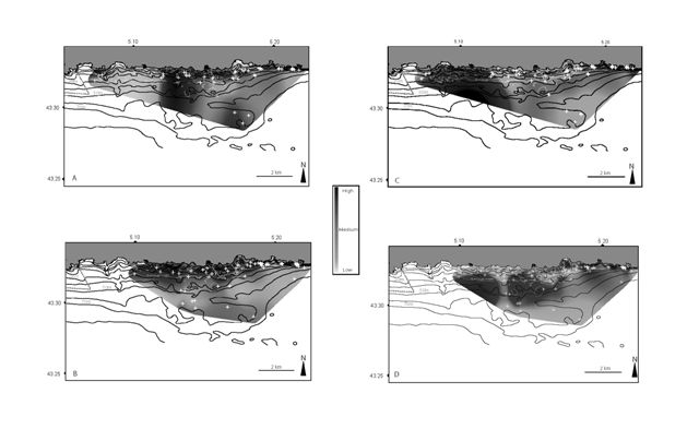
Fig. 5: Suitable Habitat in “Côte Bleue” Marine Park for adult Sparids (A & B) and for adult Scorpaenids (C & D), in spring (A & C) and in summer (B & D). White dotted line area between coast and sea delimited hard (Rock and Posidonia meadow) from soft bottom (Sand).
Source: Crec’hriou et al. Spatial patterns and GIS habitat modelling of fish in two French Mediterranean coastal areas.
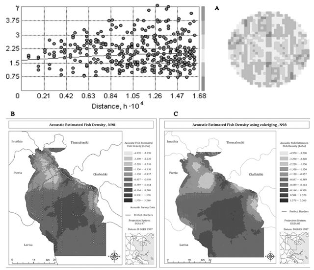
Fig. 5. Sampling survey N98: (a) Cross-Variogram (omnidirectional and exhaustive) of the Acoustic Estimated Fish Density (LnSa) using co-kriging (depth and SST), (b) Acoustic Estimated Fish Density (LnSa) using kriging and (c) using co-kriging (depth and SST).
Source: Georgakarakos & Kitsiou. Mapping abundance distribution of small pelagic species applying hydroacoustics and Co-Kriging techniques.
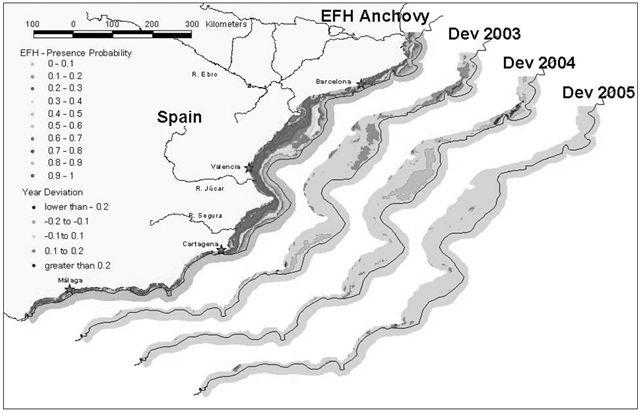
Fig. 7. EFH maps showing the predicted probability of presence of anchovy and inter-annual deviation from the general EFH model.
Source: Bellido et al. Identifying Essential Fish Habitat for small pelagic species in Spanish Mediterranean waters.
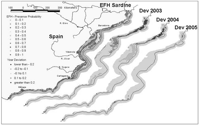
Fig. 8. EFH maps showing the predicted probability of presence of sardine and inter-annual deviation from the general EFH model.
Source: Bellido et al. Identifying Essential Fish Habitat for small pelagic species in Spanish Mediterranean waters.
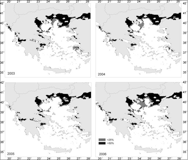
Fig. 6. Map of areas representing anchovy potential spawning habitat in Greek waters based on the GAM model from the North Aegean Sea Grey colour: >25%; black colour: >50% probability of spawning.
Source: Schismenou et al. Modeling and predicting potential spawning habitat of anchovy (Engraulis encrasicolus) and round sardinella (Sardinella aurita) based on satellite environmental information.
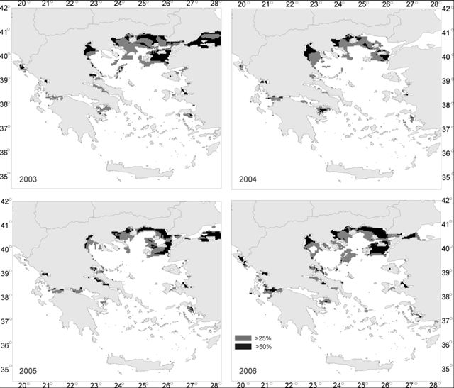
Fig. 7. Map of areas representing round sardinella potential spawning habitat in Greek waters based on the GAM model from the North Aegean Sea Grey colour: >25%; black colour: >50% probability of spawning.
Source: Schismenou et al. Modeling and predicting potential spawning habitat of anchovy (Engraulis encrasicolus) and round sardinella (Sardinella aurita) based on satellite environmental information.
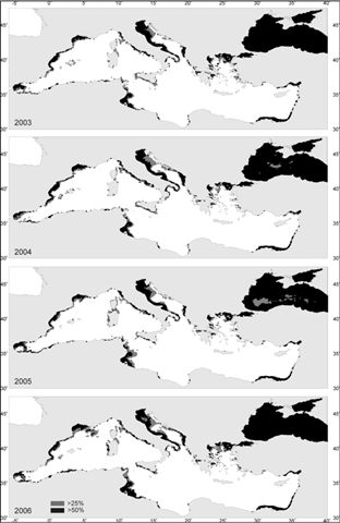
Fig. 8. Mediterranean Sea. Map of areas representing anchovy potential spawning habitat based on the GAM model from the North Aegean Sea Grey colour: >25%; black colour: >50% probability of spawning.
Source: Schismenou et al. Modeling and predicting potential spawning habitat of anchovy (Engraulis encrasicolus) and round sardinella (Sardinella aurita) based on satellite environmental information.
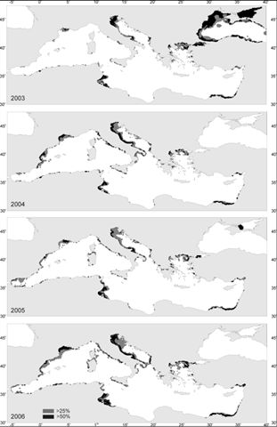
Fig. 9. Mediterranean Sea. Map of areas representing round sardinella potential spawning habitat based on the GAM model from the North Aegean Sea Grey colour: >25%; black colour: >50% probability of spawning.
Source: Schismenou et al. Modeling and predicting potential spawning habitat of anchovy (Engraulis encrasicolus) and round sardinella (Sardinella aurita) based on satellite environmental information.
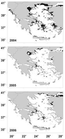
Fig. 3. Geographic distribution of regions post-classified as “juvenile” areas, by applying the DFA for a grid of spots within the Greek Seas, for June 2004-2006.
Source: Tsagarakis et al. Habitat discrimination of juvenile sardines in the Aegean Sea using remotely-sensed environmental data.
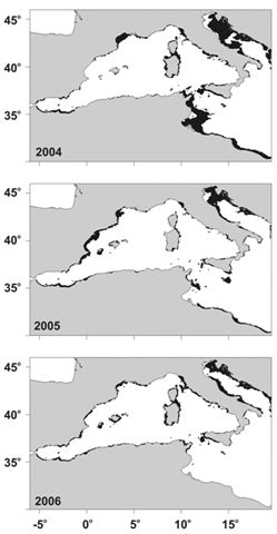
Fig. 4. Geographic distribution of regions post-classified as “juvenile” areas, by applying the DFA for a grid of spots within the Western Mediterranean Sea, for June 2004-2006.
Source: Tsagarakis et al. Habitat discrimination of juvenile sardines in the Aegean Sea using remotely-sensed environmental data.
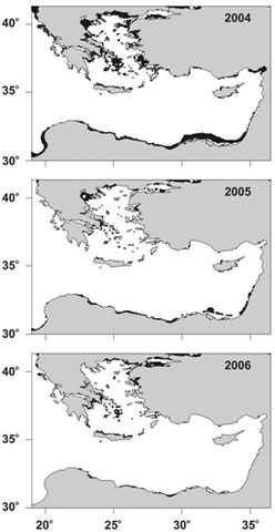
Fig. 5. Geographic distribution of regions post-classified as “juvenile” areas, by applying the DFA for a grid of spots within the Eastern Mediterranean Sea, for June 2004-2006.
Source: Tsagarakis et al. Habitat discrimination of juvenile sardines in the Aegean Sea using remotely-sensed environmental data.
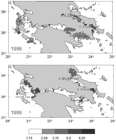
Fig. 6. Distribution maps of anchovy according to the ln of NASC (Nautical Area Scattering Coefficient in m2/nm2) for June 1998 and 1999, respectively. Kriging was used as the interpolation method (spacing 1 nm, spherical variogram model and anisotropy).
Source: Giannoulaki et al. Modelling the presence of anchovy Engraulis encrasicolus in the Aegean Sea during early summer, based on satellite environmental data.
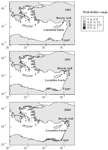
Fig. 7. Eastern Mediterranean Sea: Map of the probability for anchovy potential presence based on GAM model from Aegean Sea. GIS resolution used for prediction was 4 km of mean monthly satellite values from a. June 2004, b. June 2005 and c. June 2006.
Source: Giannoulaki et al. Modelling the presence of anchovy Engraulis encrasicolus in the Aegean Sea during early summer, based on satellite environmental data.
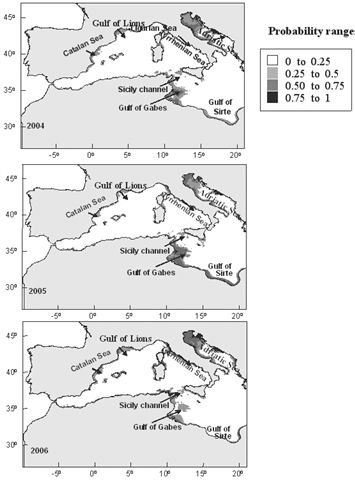
Fig. 8. Western Mediterranean Sea: Map of the probability for anchovy potential presence based on GAM model on records from Aegean Sea. GIS resolution used for prediction was 4 km of mean monthly satellite values from a. June 2004, b. June 2005 and c. June 2006.
Source: Giannoulaki et al. Modelling the presence of anchovy Engraulis encrasicolus in the Aegean Sea during early summer, based on satellite environmental data.
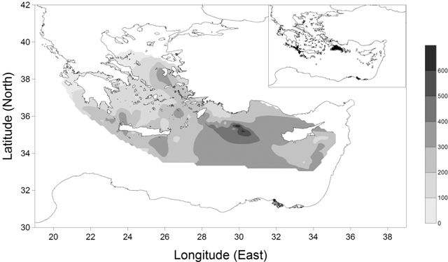
Fig. 5. Map of swordfish distribution during the peak spawning period, based on the GAM predictions. Abundance is expressed in terms of kg/1000 hooks. Observations are depicted on the small map on the upper right corner; the diameter of the circles is proportional to the CPUE value.
Source: Tserpes et al. Distribution of swordfish in the eastern Mediterranean, in relation to environmental factors and the species biology.
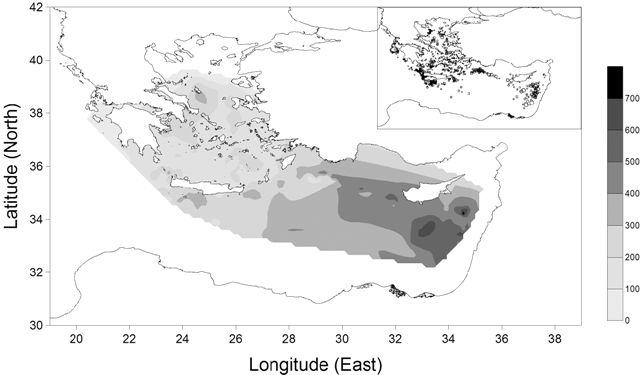
Fig. 6. Map of swordfish distribution during the migration period, based on the GAM predictions. Abundance is expressed in terms of kg/1000 hooks. Observations are depicted on the small map on the upper right corner; the diameter of the circles is proportional to the CPUE value.
Source: Tserpes et al. Distribution of swordfish in the eastern Mediterranean, in relation to environmental factors and the species biology.
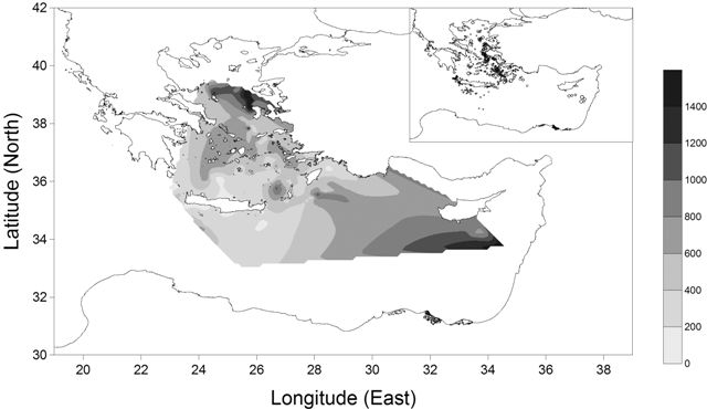
Fig. 7. Map of swordfish distribution during the winter feeding period based on the GAM predictions. Abundance is expressed in terms of kg/1000 hooks. Observations are depicted on the small map on the upper right corner; the diameter of the circles is proportional to the CPUE value.
Source: Tserpes et al. Distribution of swordfish in the eastern Mediterranean, in relation to environmental factors and the species biology.
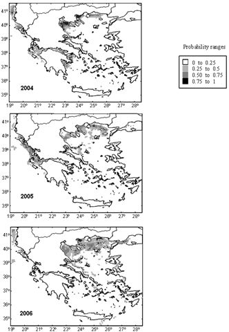
Fig. 4. Map of the probability of potential M. leidyi presence in the Greek region, based on GAM model from northern Aegean Sea. GIS resolution used for prediction is 4 km of mean monthly satellite values from a. June 2004, b. June 2005 and c. June 2006.
Source: Siapatis et al. Modelling potential habitat of the invasive ctenophore Mnemiopsis leidyi in Aegean Sea.
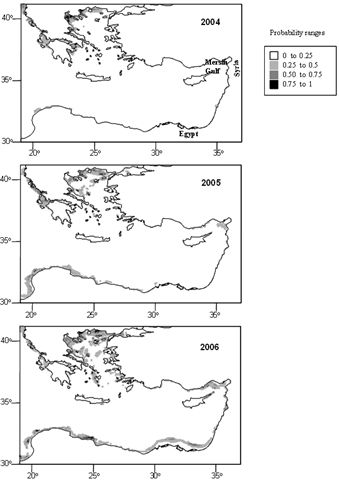
Fig. 5. Eastern Mediterranean Sea: Map of the probability of potential M. leidyi presence based on GAM model from Aegean Sea. GIS resolution used for prediction was 4 km of mean monthly satellite values from a. June 2004, b. June 2005 and c. June 2006.
Source: Siapatis et al. Modelling potential habitat of the invasive ctenophore Mnemiopsis leidyi in Aegean Sea.
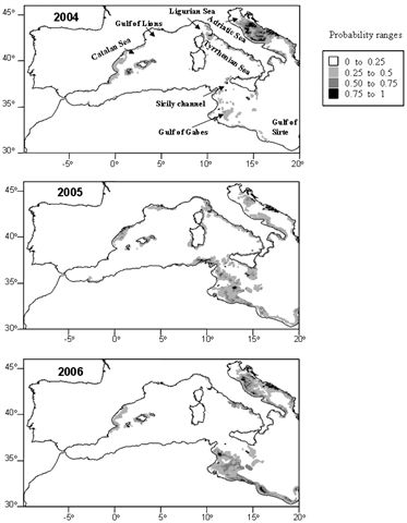
Fig. 6. Western Mediterranean Sea: Map of the probability of potential future M. leidyi presence based on GAM model on records from Aegean Sea. GIS resolution used for prediction was 4 km of mean monthly satellite values from a. June 2004, b. June 2005 and c. June 2006.
Source: Siapatis et al. Modelling potential habitat of the invasive ctenophore Mnemiopsis leidyi in Aegean Sea.